Products
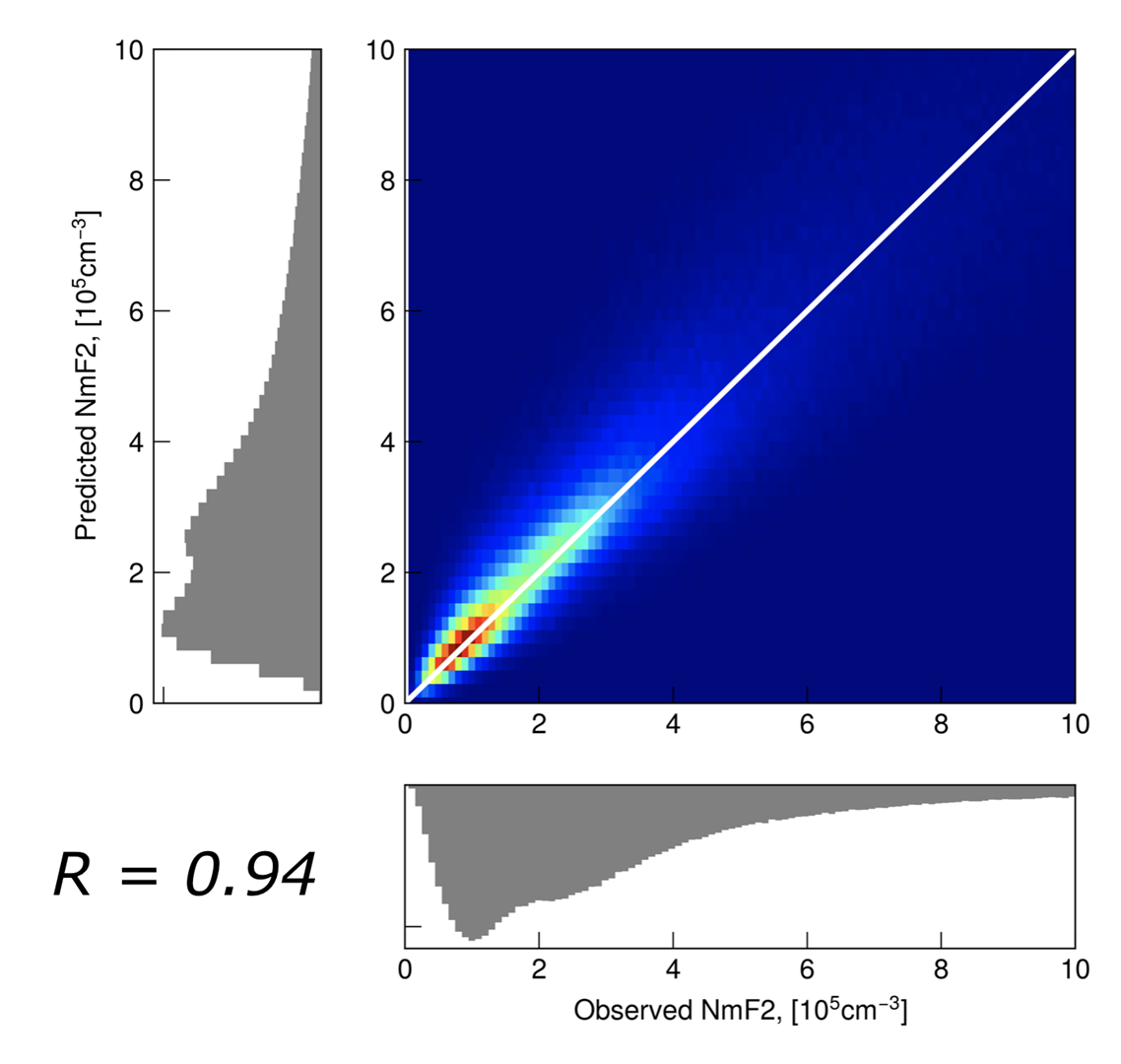
2D histogram of observed versus predicted NmF2
The corresponding distributions are shown in panels under the axes. The model adequately reproduces the NmF2 values, and closely captures the distribution shape.
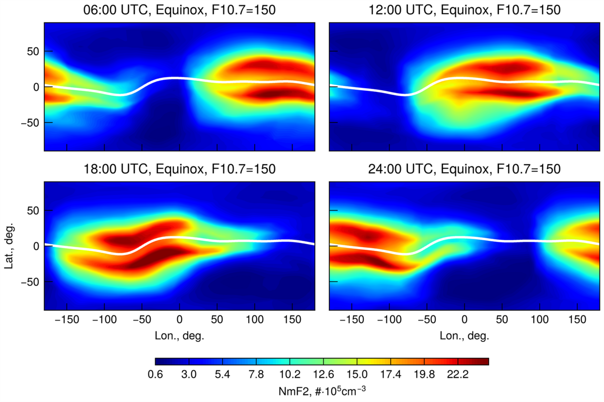
Diurnal variability of NmF2 for 2019 (vernal equinox), under F10.7=150
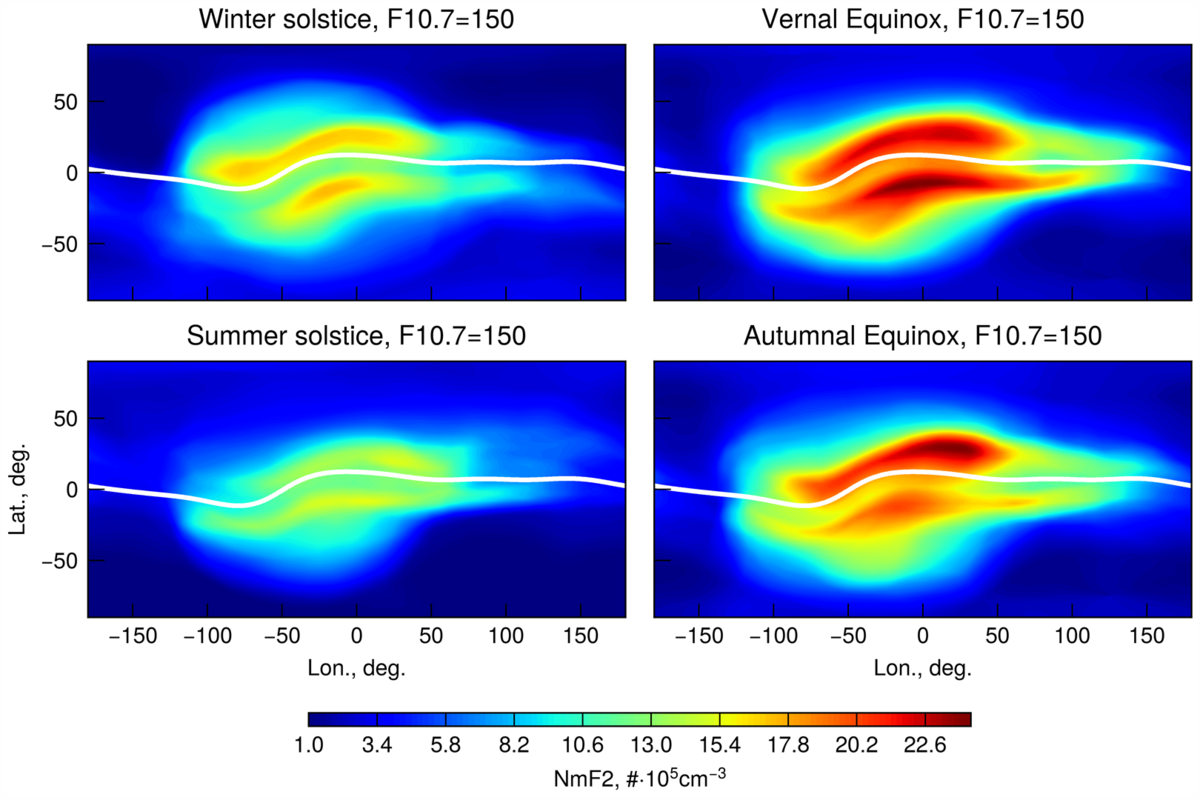
Seasonal variability of NmF2
The synthetic model run was conducted for F10.7=150, 15:00 UTC, for different DOY, corresponding to the northern and southern solstices and vernal and autumnal equinoxes.
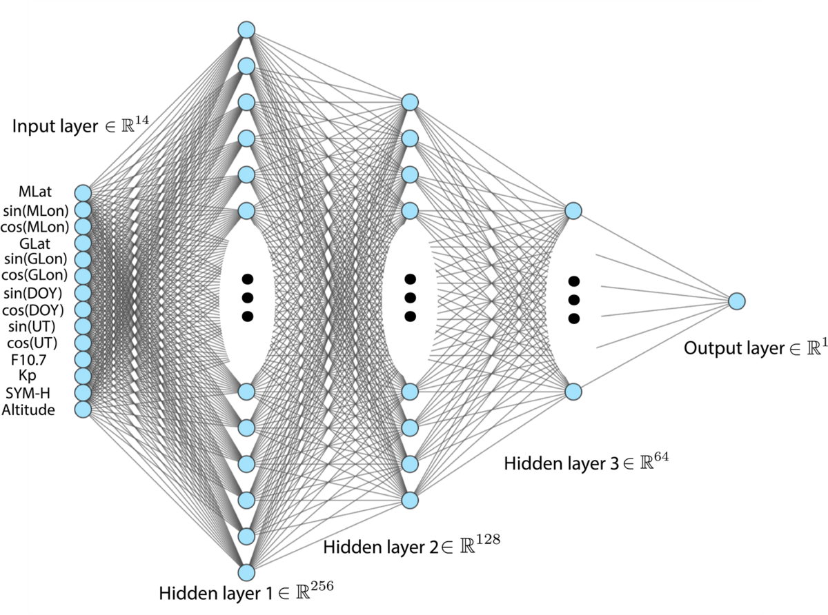
Neural network architecture
The input layer consists of 14 parameters, including position, local time, season and indices of solar and geomagnetic activity. The network has 3 hidden layers with 256, 128 and 64 neurons, respectively. Output is the normalized electron density.
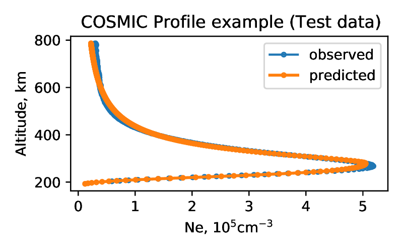
COSMIC profile
An example of the COSMIC profile from the test set, reconstructed using the neural network model.
Neural Network Model
Example run of the neural network model, showing the diurnal variation of electron density at 400 km. The run was conducted for F10.7=150, during vernal equinox (DOY=84).
Example run of the neural network model, showing the variation of electron density with changing altitude. The two EIA crests appear at around 200 km, become most instense at ~350 km, and then slowly fade and merge into one at higher altitudes. The run was conducted for F10.7=150, during vernal equinox (DOY=84), 12:00 UTC. Geomagnetic equator is shown with a bold silver line.
Example run of the neural network model, showing the seasonal variation of electron density at 400 km. The run was conducted for F10.7=150, by changing DOY from 001 to 365.
VTEC diurnal evolution model
Example run of the neural network model for generating ionospheric Vertical Total Electron Content (VTEC) over a 24-h cycle. The run was conducted with F10.7 = 125.6 and DOY=1.